1. Introduction to astrophysics and cosmology
1.1. What it is Astrophysics?
It is worthwhile to review the ethimology of the categories mainly studied in this field: “astronomy”, “astrophysics” and “cosmology”. The distinction between these three categories is by far arbitrary, although it shows partially the historical development of this branch of science.
These three categories may be defined as follows:
Astronomy: It is devoted to the stuy and determination of the measurements of coordinates, proper motions, brightness, spectra of any object in space.
Astrophysics: It is fouced on analyzing the behavior of any object in space, but applying physical theories to understand observations and make predictions.
Cosmology: It studies the large-scale structure of the Universe, but also its origin, composition and evolution.
Of course, once these cateogires have been defined, the reader might disagree with the definitions, the number of categories, or even the use of categories. Indeed, nowadays these categories are completely intertwined. Astronomy comes first as it is the oldest one, but then cosmology is the big jump that came in the mid 1900s. But it is imposible to not apply physics to understand everything that is being observed in the sky. Thus, we can certainly use “astrophysics” in its wide and general definition.
A very important aspect in this field of science is that it is extremely hard (although not impossible Cosmic Dust Laboratory) to perform experiments, as most of the physical conditions are (nowadays) unacheivable on Earth laboratories. Hence, astrophysics is focused on observations and data analysis. Observations mainly come from photons, but in the recent years there has been clear advances towards multi-messenger astronomy by neutrinos (e.g. Aartsen et al. 2013, 2014, 2017) and gravitational waves (e.g. Abbott et al. 2017, 2019).
Nonetheless, astrophysics also offers a unique framework to test most of the different branches from physics: mechanics, electromagnetism, magneto-hydrodynamics, thermodynamics, statistical physics, special and general relativity, atomic and molecular physics, … Hence, it is necessary to understand the different temperature-, length- and timescales that are involved, and at which extent the different quantum and/or relativistic effects take place. In return, we have en excellent benchmark to test recent theories such as:
New matter states and new quantum particles
The vacuum
Intense magnetic fields
General Relativity tests
Overall, these lectures will not be versed neither in positional astronomy, neither on pre-planck cosmology, but rather in providing a complete picture of all the aspects involved in astrophysics.
1.2. A brief historical summary
As it has been already mentioned, astrophysics is both one of the oldest and newest scientific disciplines. Hence, it is useful to review all the advances in the field across human history. We can review them in terms of specific epochs:
Epoch 1: During this first epoch, which started around 4,000 BC, and ended around 600 BC, mithology and science are extremely correlated. During this epoch, mistic problems (astrology) and the need for orientation and agriculture enhances studies on the sky. We can observed in the Neolithic period (e.g. Szucs-Csillik & Maxim 2019) representations of constellations, the Chinese culture is well-known for the elaboration of calendars and register of astronomical events (e.g. Sun 2009), the Egyptian culture focused on the orientation of the pyramids and the observation of the Syrius star (e.g. Haack 1984, Rawlins & Pickering 2001, Nell & Ruggles 2014), and the Babylonians also elaborated calendars and the so-called “Saros Cycle” (solar eclipses, e.g. Goldstein 2002).
Epoch 2: This epoch (between 600 BC and 200 AD) occurs mainly in Greece. Thanks to philosophers such as Thales of Miletus1 or Pythagoras2, the first scientific formulations came into play. For example, the first geometrical models for the Universe were proposed:
Geocentric model: Defended, among many others, by Eudoxus of Cnidus3, Plato4 and Aristotle5.
Epicylic model: Porposed by Claudius Ptolemaeus6, which introduces some modifications in the celestial motions with respect to the goecentric model.
Heliocentric model: Defended by Aristarchus of Samos7 and Seleucus of Seleucia8.
Additionally, the first star catalogs are published:
The Hipparchus9 catalog, containing the position and magnitud of around 850 stars.
The Ptolemaus catalog, also known as the Almagest, containing over 1,100 stars, and whose use extent to the Middle Age.
Epoch 3: This epoch lasted between 200 and 1500 AD, being mainly focused on the Middle Age. In the year 964, the arab astronomer al-Sufi10 published a catalog containing different nebulae. During this period of time, we have reports of observing two supernovae in 1006 (reported by Chinese, Japanese and Egyptian astronomers) and in 1054 (observed by Chinese, Japanese and Amerindian cultures). In Spain, during the XIII century, the so-called Tablas Alonsíes11 were elaborated, containing all celestial observations between 1263 and 1272 AD of the Toledo’s night sky.
Epoch 4: Between 1500 and 1870 AD, this epoch is characterized mainly by an opening to different theories. In a very first place, we can highlight the early works from Copernicus, Galileo, Kepler and Newton:
Copernicus12 returned to the Heliocentric model already postulated in the Ancient Greece.
In 1608, the telescope is invented in Netherlands, and Galileo13 used it to observe four satellites around Jupyter, solar spots, Venus phases, mountains in the moon, etc.
Two supernovae events were observed, in 1572 by Brahe14 and in 1604 by Kepler15, as well as comets (in 1577 by Brahe) and the variable star Mira Ceti (in 1596 by Fabricius16). These events were milestones in shifting from the Geocentric to the Heliocentric model.
Between 1609 (first two) and 1619 (the third one), Kepler published the so-called “Kepler’s Laws of Planetary Motion”.
Newton17 formulated the his Theory of Gravity and Universal Gravitation in this famous Principae (1687), unifying Kepler’s laws and the free-fall of objects. He also worked on understading light and its composition.
In 1676, Rømer17 measured the speed of light to a first approximation (see Shea 1998).
In 1705, Halley18 predicted that the comet observed in 1682 would be observed again in 1758.
In a second place, we can also highlight the advancements beyond the telescope that came with:
The advancements made by Wollaston19, Fraunhofer20 and Kirchhoff21 between 1800 and 1860 resulted in the development of spectroscopy, allowing for instance the determination of the chemical composition of the Sun by its absorption lines.
The development of photography and its application to astronomy by Draper22 in 1840.
Finally, it is important to mention the work by Argelander23, who published between 1859 and 1862 the largest catalog, Bonner Durchmusterung, of stars (~324,000) without the use of photography.
Epoch 5: This epoch corresponds to the XX century, characterized by new conceptual and observational horizons. Einstein24 postulated his theories of Special (Einstein 1905) and General (Einstein 1916) Relativity, which led to new models of our understanding of the Universe, such as those proposed by de Sitter25, Friedmann26 and Lemaître27, and also lead to the formulation of black hole formation theories by Schwarzschild28 (1916) (for a non-rotating, uncharged object), by Reissner29 (1916) (for a non-rotating, charged object), by Kerr30 (1963) (for a rotating, uncharged object) and by Newman31 et al. (1965a,b) (for a rotating, charged object).
In early 1910s, the independent works by Hertzsprung32 (1911) and Russell33 (1913, 1914a,b) found a correlation between the color and brightness of the stars, leading to the so-called “Hertzsprung-Russell diagram” (H-R diagram). The early works by Eddington34 (1916, 1918, 1919, 1922, 1926) led to the stellar evolution theory.
During this epoch, the core idea of “Universe” was also revisited, moving away from the theory of Universes as Isles by Kant35, thanks to the a more robust classification of the observed nebulae by the New General Catalogue (NGC, Dreyer 1888). Thus, in 1920 the *Great Debate" between Shapley36 and Curtis37 on tha size of the Universe and the existence of other galaxies. While both astronomers use correct arguments, the idea defended by Curtis (that some of the observed nebulae were independent galaxies) was proven true by Hubble38 (e.g. Hubble 1926), by meausring Cepheids in Andromeda. Later on, Hubble works proved that the Universe was expanding as galaxies were redshifting (Hubble 1929).
Several advancements on the field of subatomic and quantum physics led to several predictions, such as the existence of neutrons (Rutherford 2020), pions (Yukawa 1942), neutrinos (Pauli letter), quarks (Gell-Mann 1964, Zweig 1964), the Higgs boson (Higgs 1964a,b, 1966) and the Supersymmetry (SUSY) theory (e.g. Salam & Strathdee 1974). The majority of these predictions were confirmed by observations and experiments (Chadwick 1932, 1933, Lattes et al. 1947, Cowan et al. 1956, Bloom et al. 1969, Breidenbach et al. 1969, Herb et al. 1977, Abrams et al. 1974, Augustin et al. 1974, CERN collaboration 2012).
It is also important to highlight the advancements in the field of astronomical observations by observing radio, X-ray and $\gamma$-ray radiation. Radio wavelength observations allowed the discovery of the Cosmic Microwave Background radiation (Penzias & Wilson 1965) or pulsars (Hewish et al. 1968). Thanks to the technology development of the Cold War, this epoch was characterized by the first confirmation of x-ray emission coming from outside the Solar System ([Giacconi et al. 1962](Evidence for x Rays From Sources Outside the Solar System)). Finally, it is worthwhile to mention the detection of $\gamma$-rays through the Vela USA military satellites, originally dsegined the $\gamma$-ray burst from nuclear bomb detonations, but eventually detecting the $\gamma$-ray emission from our own Galaxy (Klebesadel, Strong and Olson 1973).
Epoch 6: It is difficult to explain this epoch as, from our point of view, is the one we are currently leaving. We can highlight three major aspects: the increase of statistics and quality of the data, and the multi-messenger astronomy. However, this major break in astronomy also push to the limits some of our assumed theories for the formation of the Universe. As of 2025, it is difficult to assess such impact.
Ground-based observatories have contributed significantly in astronomy. Surveys such as Sloan Digital Sky Survey (SDSS39, York et al. 2000), have signficantly increased astronomy in many fronts: the imaging data covers around 35,000 square degrees (see the official website for more details); the supernovae survey containing over 900 SNe events spectroscopically confirmed (see the official website for more details); the spectra of over 2,800,000 galaxies, 1,020,000 stars and 960,000 quasars (see the official website for more details); spatially resolved spectroscopic observations of around 10,000 galaxies (see the official website for more details) and many other added-value products (see the offical website for more details). Although SDSS was a singificant revolution back in the day, now the Dark Energy Spectroscopy Instrument(DESI40, DESI collaboration et al. 2022) is pushing the limits to a new standard, as the first data release (DR1) has provided spectroscopic information for over 13,100,000 galaxies, 4,000,000 stars and 1,600,000 quasars (DESI collaboration et al. 2025). There has been also significant advancements in other surveys, such as the search for exoplanets with Calar Alto high-Resolution search for M dwarfs with Exoearths with Near-infrared and optical Echelle Spectrographs (CARMENES41, Quirrenbach et al. 2016). Other important highlights come from the Very Large Telescope (8.2m, VLT), the Gran Telescopio de Canarias (10.4m, GTC) or the future Extremely Large Telescope (39m, ELT), and their instrumentation. Radio observations have also been enhanced by facilities such as the Atacama Large Millimeter Array (ALMA, Kurz & Shaver 1999).
In terms of space-based observatories, have been proben to as essential as their ground-based counterparts. Missions such as Planck42 (see Planck Collaboration 2008 for more details) have been crucial in our understanding and modeling of the Universe (e.g. Planck Collaboration et al. 2014a,b, 2016a,b, 2020a,b). The infrardd regime, limited by the sky absorption, also experienced a signficant improvement thanks to missions such as the Infrared Space Observatory (ISO, Kessier et al. 1996), the Spitzer Space Telescope (Spitzer, Werner et al. 2004), the AKARI mission (Murakami et al. 2007), the Herschel Space Observatory (Herschel, Pilbratt et al. 2010) or the James Webb Space Telescope (JWST, Gardner et al. 2910). The optical and near-ultraviolet regime has been exploited in many other ways by the launched of the Hubble Space Telescope (HST, Turnsheck et al. 1990). X-rays observations have been also increased thanks to the Chandra X-ray Observatory (CXO, Weisskopf et al. 2002) and the XMM-Newton Observatory (Jansen et al. 2001).
In the realm of our models and theories for understanding the Universe, this epoch has been characterized by the enigmas, and the remaining open questions. The Hubble Constant has been a matter of discussion, as different techniques provides different measurements, leading to the so-called “Hubble Tension” (e.g. Di Valentino et al. 2021, Efstathiou 2021, Hu et al. 2024, Verde, Schnöneberg & Gil-Marín 2024). The amplitude of the matter fluctuations has also been under debate (e.g. Planck Collaboration et al. 2020, Adil et al. 2024). Our understanding of galaxy formation, from Dark Matter halos following a hierarchal growth and capturing pristine gas (e.g. Cole et al. 2000, Springel et al. 2018, Martizzi et al. 2019), has some problemas such as the “Missing Satellite Problem” (e.g. Nashimoto et al. 2022) or the “Too-Big-To-Fail Problem” (e.g. Ogiya & Burkert 2015). Overall, both our comoslogical model and theory for galaxy formation have several caveats and problems that suggest further research (e.g. Bullock & Boylan-Kolchin 2017, Efstathiou 2025).
Lastly, it is important to mention that this new epoch is characterized also by a multimessenger approach: not only we can observe (and retrieve information), from photons, but also from other sources. Neutrinos were proposed several decades ago as a new window of observations (Greisen 1960), but they have become a clear reality thanks to the IceCube Neutrino Observatory (Aartsen et al. 2013, 2014, 2017). In a similar fashion, cosmic rays (less specific than neutrinos), have also been proposed as a window for observations (e.g. Sommers & Westerhoff 2009), which is now being exploited with observatories such as the Pierre Auger Observatory (Abraham et al. 2004, Pierre Auger Collaboration 2015). $\gamma$-rays, the most energetic form of electromagnetic radiation, have been also used to observe the Universe with facilities such as the Cherenkov Telescope Array (CTA, Actis et al. 2011) or the Fermi Gamma-ray Space Telescope (Fermi, Ackermann et al. 2015, 2016). Gravitational waves, already predicted in the late 1910s as a natural outcome from General Relativity (Einstein 1916, 1918, Eddington 1922), were finally detected in the 2010 decade thanks to the Laser Interferometer Gravitational-Wave Observatory (LIGO) and the Virgo-inferferometer (Virgo) in 2016 (Abbott et al. 2016), with more detections in the next years (e.g. Abbott et al. 2017, 2019).
While neither complete nor exhaustive, this schematic overview gives us a clear idea on both the importance of astronomy in human history and the development that has been experienced over the last centuries.
1.3. Orders of magnitude
Astrophysics are described with several (if not all) measurement scales due to the large variety of physical processes involved. This is highlighted in the different units used across the field. However, before addressing such variety of units, it is important to review two fundamental parts: the main units used and the physical constants involved.
As we are thaught at schools, when dealing with science the metric system that we should be using is the International System (SI, learn more). These units are not arbritary, but rather taken from Universal constants. The problem: in astrophysics we do not generally used such units, but rather the centimeter-gram-second (CGS) system of units (or a mixture between CGS and SI). Thus, a comparative table of the fundamental units should always be at hand (such as the Table 1.1).
Table 1.1. Basic physical properties and their corresponding units depending on the system.| Base property | Property symbol | SI unit | CGS unit | Conversion factor |
|---|---|---|---|---|
| Time | t | second (s) | second (s) | - |
| Length | l,r | meter (m) | centimeter (cm) | 10$^2$ cm = 1 m |
| Mass | m,M | kilogram (kg) | gram (g) | 10$^3$ g = 1 kg |
| Electric current | i,I | ampere (A) | statampere (statA) | 2.9979245$\cdot 10^7$ statA = 1 A |
| Temperature | T | kelvin (K) | kelvin (K) | - |
| Amount of substance | n | mole (mol) | mole (mol) | - |
| Luminous intesity | I$_{\nu}$ | candela (cd) | - | - |
The choice of a unit systm has deeper problems rather than the need to convert the final number: the change of equations. For instance, in natural units (h = c = 1), most of the equations do not account for those terms as they are set to 1, hence the conversion is more tricky. With that in mind, we can take a look at how important physical (see Mohr et al. 2025 for a full version of all them) constants change:
Table 1.2. Most used physical constants and their change due to the unit system.| Physical constant | Symbol | SI value | CGS value |
|---|---|---|---|
| Planck constant | h | $6.62607015\cdot 10^{-34}$ J$\cdot$s | $6.62607015\cdot 10^{-27}$ erg$\cdot$s |
| Speed of light | c | $2.99792458\cdot 10^{8}$ m$\cdot$s$^{-1}$ | $2.99792458\cdot 10^{10}$ cm$\cdot$s$^{-1}$ |
| Vacuum magnetic permeability | $\mu_{0}$ | $1.25663706212\cdot 10^{-6}$ N$\cdot$A$^{-2}$ | $1.25663706212\cdot 10^{-15}$ dyn$\cdot$statA$^{-2}$ |
| Elementary charge | e | $1.602176634\cdot 10^{-19}$ C | $1.602176634\cdot 10^{-12}$ statA$\cdot$s |
| Fine-structure constant | $\alpha$ | $7.2973525693\cdot 10^{-3}$ | $7.2973525693\cdot 10^{-3}$ |
| Rydberg Energy | h$\cdot$c$\cdot$R$_{\infty}$ | $2.179872361\cdot 10^{-18}$ J | $2.179872361\cdot 10^{-11}$ erg |
| Electron mass | m$_{e}$ | $9.1093837015\cdot 10^{-31}$ kg | $9.1093837015\cdot 10^{-31}$ g |
| Boltzmann Constant | k | $1.380649\cdot 10^{-23}$ J$\cdot$K$^{-1}$ | $1.380649\cdot 10^{-16}$ erg$\cdot$K$^{-1}$ |
| Gravitational constant | G | $6.6743\cdot 10^{-11}$ m$^{3}\cdot$kg$^{-1}\cdot$$s^{-2}$ | $6.6743\cdot 10^{-8}$ cm$^{3}\cdot$g$^{-1}\cdot$$s^{-2}$ |
In order to get an idea of the variety of orders of magnitude involved, let us analyze with practical examples. We show in Table 1.3 examples of those orders:
Table 1.3. Orders of magnitude involved in astrophysics in different physical properties.| LENGTH | |||
|---|---|---|---|
| Example | Value | SI value | Reference |
| Proton radius | $\sim$0.87 fm | $\sim 8.7\cdot 10^{-16}$ m | Guth (1987); Brandenberger (2021) |
| Optical wavelength | $\sim$500 nm | $\sim 5\cdot 10^{-7}$ m | Bessell (2004) |
| Ground-based telescope mirror | $\lesssim 39$ m | $\lesssim 39$ m | Extremely Large Telescope |
| Neutron star radii | $\sim 10$ km | $\sim 10^{4}$ m | Abbott et al. (2018) |
| Distance to the closest star | 1.295 pc | $3.9965\cdot 10^{16}$ m | van Leeuwen (2007) |
| Galaxy radii | $\sim 10$ kpc | $\sim 3.0857\cdot 10^{20}$ m | Sparke & Gallagher (2007) |
| Distance to Andromeda | $\sim 738$ kpc | $\sim 2.28 \cdot 10^{22}$ m | Wagner-Kaiser et al. (2015 |
| Galaxy cluster radii | $\sim 100$ Mpc | $\sim 3.01\cdot 10^{24}$ m | Tully et al. (2014) |
| Observable Universe | $\sim 14$ Gpc | $\sim 4.32\cdot 10^{26}$ m | Gott et al. (2005) |
| TIME | |||
|---|---|---|---|
| Example | Value | SI value | Reference |
| Cosmic inflation duration | $\sim 10^{-36}$ s | $\sim 10^{-36}$ s | Bernauer et al. (2010); Karr et al. (2020) |
| Core-collapse Supernovae explosition | $\lesssim 0.3$ s | $\lesssim 0.3$ s | Saito et al. (2022) |
| Neutron-decay timescale | $\sim 880$ s | $\sim 880$ s | Planck Collaboration et al. (2018) |
| Earth’s revolution | $\sim 1$ yr | $\sim 3.1557 \cdot 10^{7}$ s | Astronomical Almanac of the Year 2017 |
| Cosmic Microwave Background43 | $\sim 3.5\cdot 10^{5}$ yr | $\sim 1.10376\cdot 10^{13}$ s | Hu & Dodelson (2002) |
| Sun’s lifetime expectation | $\sim 10$ Gyr | $\sim 3.154\cdot 10^{17}$ s | Mowlavi et al. (2012) |
| Age of Universe | $\sim 13.8$ Gyr | $\sim 4.532\cdot 10^{17}$ s | Planck Collaboration et al. (2018) |
| MASS | |||
|---|---|---|---|
| Example | Value | SI value | Reference |
| Oxygen atom | 15.999 m$_{u}$ | $2.6567\cdot 10^{-26}$ kg | Wieser & Coplin (2011) |
| Halley’s comet mass | $\sim 2.2\cdot 10^{17}$ g | $\sim 2.2\cdot 10^{14}$ kg | Hughes (1985) |
| Earth’s mass | $\sim 5.972 \cdot 10^{27}$ g | $\sim 5.972 \cdot 10^{24}$ kg | Folkner & Williams (2008) |
| Solar mass | 1 M$_{\odot }$ | $1.9891\cdot 10^{30}$ kg | Pitjeva & Pitjev (2012) |
| R136a1 mass | $\sim 315$ M$_{\odot}$ | $\sim 6.266\cdot 10^{32}$ kg | Crowther et al. (2016) |
| Galaxy stellar mass range | $\sim 10^{6} - 10^{12}$ M$_{\odot}$ | $\sim 10^{36} - 10^{42}$ kg | Furlong et al. (2015) |
| Cluster masses | $\sim 10^{14} - 10^{15}$ M$_{\odot }$ | $\sim 10^{44} - 10^{45}$ kg | Andreon (2016) |
| TEMPERATURE | |||
|---|---|---|---|
| Example | Value | SI value | Reference |
| Cosmic Microwave Background temperature | $\sim 2.755$ K | $\sim 2.755$ K | Muller et al. (2013) |
| Atomic gas temperature | $\sim 100$ K | $\sim 100$ K | Dutta et al. (2019) |
| Sun surface temperature | T$_{sup,\odot }$ | $\sim 5772$ K | Prsa et al. (2016) |
| AGN accretion disk temperature | $\sim 10^{5}$ K | $\sim 10^{5}$ K | Cheng et al. (2019) |
| Sun inner temperature | T$_{c,\odot }$ | $\sim 1.5 \cdot 10^{7}$ K | Bahcall, Serenelli & Basu (2006) |
In summary, as clearly drawn from Table 1.3 working in Astrophysics means dealing with different scales, although most of the times, when studying a particular field, the range in the scales becomes narrower. Nonetheless, it is extremely useful to bear in mind the different scales.
1.4. Precision in the measurements
Once we have a clear idea on the scales involved, we can discuss how precise we can get when observing the Universe. The answer to the question is so far very complex. On the one hand, the number of physical processes and assumptions needed to understand observations implies that the precision in the estimations cannot drop down from 1/10th of estimated qunatity. For instance, the stellar mass or star formation rates in galaxies are measured with a relative uncertainty of $\sim$ 0.1-0.3 dex, which in absolute terms is quite a number (e.g. Feulner et al. 2005, Davé 2008, Kaushal et al. 2024). Gas-phase metallicities in the ISM are derived with similar relative uncertainties (e.g. Pérez-Montero 2017, Maiolino & Mannucci 2019, Dors et al. 2020).
However, not all the scenarios explored in astrophysics can be addressed with such high uncertainties. That is for the instance the case of neutrino oscillations, originally reported by Davis, Harmer & Hoffman (1968) and Bahcall, Bahcall & Shaviv (1968), which has been confirmed by other experiments (e.g. Fukuda et al. 1998, Aguilar et al. 2001, Ahn et al. 2003). As hinted by the Comic Background Explorer (COBE; [Smoot et al. 19922]https://ui.adsabs.harvard.edu/abs/1992ApJ…396L…1S/abstract), Efstathiou, Bond & White 1992, Wright et al. 1992), but clearly shown by the Wilkinson Microwave Anisotropy Probe (WMAP; Spergel et al. 2003, Hinshaw et al. 2013), the CMB deviates from the perfect blackbody spectra due to temperature fluctuations ($\Delta T \sim 10^{-5} T$; Hinshaw et al. 1996), which correlate with the large-scale matter distribution (e.g. Boughn & Crittenden 2004), but are likely originated from inflation quantum perturbations (e.g. Gaztañaga & Sravan Sumar 2024). Another example lies on the detection of gravitational waves, as the wave strain44 is in the order of $\sim 10^{-21}$ for the events45 detected with LIGO (e.g. Abbott et al. 2016, 2017, 2019).
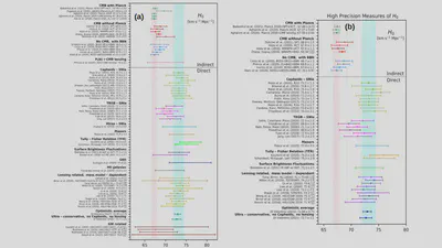
Whereas we have reviewed a great number of exemptions in which the accuracy of the measurements are critical for the reliability of the results, let us focus on a particular case, the Hubble tension. The Hubble constant ($H_{0}$ [km/s/Mpc]) . Ironically, one can find another “tension” (or better said “controversy”) when starting to address the issue of the determination of the Hubble constant (see note below). The Hubble constant has been measured through several ways, which are generally categorized by “early Universe” (if the measurement is related to the physics of the early Universe) or “late Universe” (if the measurement is related to physics in the local Universe). It is beyond the scope of this handnotes to further elaborate on the techniques (although we will address it in a future chapter), but the key message is that what initially was attributed to the uncertainty in the measurements, now it is clear that there is discrepancy among the results from the early and late Universe (see Di Valentino et al. 2021 for an excellent review). This is shown in Fig. 1 (taken from Di Valentino et al. 2021 review). In Figure 1.1 (a) we observed that the median values of $H_{0}$ from “early Universe” techniques provide different values than the others. Particularly, if we focus on the two main techniques; the Planck estimation (Planck Collaboration et al. 2020) and the SNe estimation from the SH0ES collaboration (Riess et al. 2021), we can see that the difference is already 4 to 6$\sigma$ range, which implies that is real. Thus, improving the uncertainty in our estimations has been crucial in understanding the need to possibly explore new physical scenarios.
1.5. Recommended books and articles
If the reader wants to get a better idea of the ideas highlighted in this preliminary chapter, here are some useful suggestions:
- Astronomy and History - Selected Essays O. Neugebauer, 1986. (English)
- Historia de la Fisica del Universo, E. Battaner, 2021. (Spanish)
- Encuentros temporales entre astronomía y prehistoria, J. F. Gibaja Bao & E. Pérez Montero, 2023. (Spanish)
- The International System of Units (SI) - NIST Special Publication 330, D. B. Newell & E. Tiesinga, 2019. (English)
- In the realm of the Hubble tension - a review of solutions, Di Valentino et al., 2021. (English)
- Handbook of Measurements - Benchmark for Systems Accuracy and Precision, A. A. Badiru & L. Racz, 2016. (English)
- An Intoduction to Modern Astrophysics (2nd Edition), B. W. Carroll & D. A. Ostlie, 2017. (English)
The Ancient Greek philosopher from Miletus in Ionia, Asia Minor (626/623 - 548/545 BC). ↩︎
The Ancient Greek philosopher (570 - 495 BC). ↩︎
The Ancient Greek astronomer (390 - 340 BC). ↩︎
The Ancient Greek philosopher (428/423 - 348/347 BC). ↩︎
The Ancient Greek philosopher (384 - 322 BC). ↩︎
The Greco-Roman astronomer (100-160/170 AD). ↩︎
The Ancient Greek astronomer (310 - 230 BC). ↩︎
The Ancient Greek astronomer (190 - 150 BC). ↩︎
The Ancient Greek astronomer (190 - 120 BC). ↩︎
The Persian astronomer Abd a-Rahman al-Sufi (903 - 986). ↩︎
They received their name after Alfonso X of Castile, who sponsored their creation. It was created by Toledo School of Translators, composed by several scholars, and taking advantage from previous works from Islamic astronomers. ↩︎
The Polish astronomer Nicolaus Copernicus (1473 - 1543). ↩︎
The Italian astronomer and Physicist Galileo di Vincenzo Bonaiuti de’ Galilei (1564 - 1642). ↩︎
The Danish astronomer Tycho Ottesen Brahe (1546 - 1601). ↩︎
The German astronomer Johannes Kepler (1571 - 1630). ↩︎
The Frisian astronomer Johannes Fabricius (or Johann Golsmid, 1587 - 1616). ↩︎
The Danish astronomer Ole Christensen Rømer (1644 - 1710). ↩︎ ↩︎
The English astronomer Edmond Halley (1656 - 1742). ↩︎
The English chemist and physicist William Hyde Wollaston (1766 - 1828). ↩︎
The German astronomer and physicist Joseph Ritter von Fraunhofer (1787 - 1826). ↩︎
The German physcist Gustav Robert Kirchhoff (1824 - 1887). ↩︎
The American medical doctor and amateur astronomer Henry Draper (1837 - 1882). ↩︎
The German astronomer Friedrich Wilhelm August Argelander (1799 - 1875). ↩︎
The German physicist Albert Einstein (1879 - 1955). ↩︎
The Dutch mathematician Willem de Sitter (1872 - 1934). ↩︎
The Rusian physicist Alexander Alexandrovich Friedmann (1888 - 1925). ↩︎
The Belgian priest and physicist Georges Henri Joseph Édouard Lemaître (1894 - 1966). ↩︎
The German physicist and astronomer Karl Schwarzschild (1873 - 1916). ↩︎
The German aeronatuical engineer Hans Jacob Reissner (1874 - 1967). ↩︎
The New Zealand mathematician Roy Patrick Kerr (1934). ↩︎
The American physicist Ezra Theodore Newman (1929 - 2021). ↩︎
The Danish chemist and astronomer Ejnar Hertzsprung (1873 - 1967). ↩︎
The American astronomer Henry Norris Russell (1877 - 1957). ↩︎
The Englsh physicist and astronomer Sir Arthur Stanley Eddington (1882 - 1944). ↩︎
The Prusian philosopher Emanuel Kant (1724 - 1804). ↩︎
The American astronomer Harlow Shapley (1885 - 1972). ↩︎
The American astronomer Heber Doust Curtis (1872 - 1942). ↩︎
The American astronomer Edwin Powell Hubble (1889 - 1953). ↩︎
This survey is conducted with a 2.5m f/5 modified Ritchey-Chretien wide-field altitude-azimuth telescope at the Apache Point Observatory (York et al. 2000). ↩︎
This survey is conducted with a 4m Ritchey-Chretien telescope at the Kitt Peak National Observatory (DESI collaboration et al. 2022). ↩︎
This survey is conducted with a 3.5m telescope at the Calar Alto Observatory (Quirrenbach et al. 2016). ↩︎
Planck was a satellite launched in 2009 to map the anisotropies and polarization of the Cosmic Microwave Background by measuring and imaging light in the infrared and micowave regimes. ↩︎
Time since the Big Bang. ↩︎
The amount of distance compressed or stretched due to the pass of a graviational wave. Wave strain ($h$) is a dimensionless parameter that alters the local metric (although in its more general used, is a tensor that assumes the perturbation over the metric). ↩︎
The experiment consists primarily with a laser of 4 km (LIGO), which means that the compression would be physically translated into a distance of $10^{-18}$ m, which is still les than the proton radius. ↩︎